Introduction

Over the last three months, we (Animesh and I) have been working on ImageSegmentation.jl - a collection of image segmentation algorithms written in Julia. Under the mentorship of Tim Holy, we have implemented several popular image segmentation algorithms and designed a consistent interface for using these algorithms. This blog post describes image segmentation, why it’s useful and how to use the tools in this package.

Image Segmentation is the process of partitioning the image into regions that have similar attributes. Image segmentation has various applications e.g, medical image segmentation, image compression and is used as a preprocessing step in higher level vision tasks like object detection and optical flow.

Image segmentation is not a mathematically well-defined problem: for example, the only lossless representation of the input image would be to say that each pixel is its own segment. Yet this does not correspond to our own intuitive notion that some pixels are naturally grouped together. As a consequence, many algorithms require parameters, often some kind of threshold expressing your willingness to tolerate a certain amount of variation among the pixels within a single segment.

Example

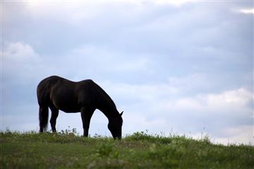
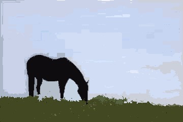
Let’s see an example on how to use the segmentation algorithms in this package. We will try to separate the horse, the ground and the sky in the image below. We will explore two algorithms - seeded region growing and felzenszwalb. Seeded region growing requires us to know the number of segments and some points on each segment beforehand whereas felzenszwalb uses a more abstract parameter controlling degree of within-segment similarity.

source

The documentation for seeded_region_growing says that it needs two arguments - the image to be segmented and a set of seed points for each region. The seed points have to be stored as a vector of (position, label) tuples, where position is a CartesianIndex and label is an integer. We will start by opening the image using ImageView and reading the coordinates of the seed points.

using Images, ImageView

img = load("horse.jpg")
imshow(img)

Hover over the different objects you’d like to segment, and read out the coordinates of one or more points inside each object. We will store the seed points as a vector of (seed position, label) tuples and use seeded_region_growing with the recorded seed points.

using ImageSegmentation
seeds = [(CartesianIndex(126,81),1), (CartesianIndex(93,255),2), (CartesianIndex(213,97),3)]
segments = seeded_region_growing(img, seeds)

All the segmentation algorithms (except Fuzzy C-means) return a struct SegmentedImage that stores the segmentation result. SegmentedImage contains a list of applied labels, an array containing the assigned label for each pixel, and mean color and number of pixels in each segment. The Result section explains how to access information about the segments.

length(segment_labels(segments))   # number of segments = 3

segment_means(segments)
#first segment's color (horse) = RGB(0.0647831,0.0588508,0.074473) = black
#second segment's color (sky) = RGB(0.793598,0.839543,0.932374) = light blue
#third segment's color (grass) = RGB(0.329876,0.357805,0.23745) = green

# for visualizing the segmentation, create an image by replacing each each label in label_map(segments) with it's mean color
imshow(map(i->segment_means(segments,i), labels_map(segments)))

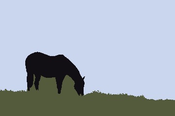
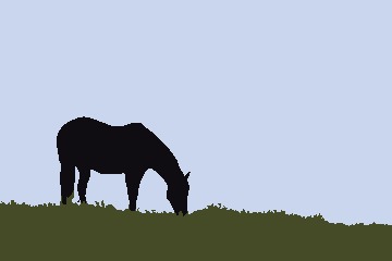
You can see that the algorithm did a fairly good job of segmenting the three objects. The only obvious error is the fact that elements of the sky that were “framed” by the horse ended up being grouped with the ground. This is because seeded_region_growing always returns connected regions, and there is no path connecting those portions of sky to the larger image. If we add some additional seed points in those regions, and give them the same label 2 that we used for the rest of the sky, we will get a result that is more or less perfect.

seeds = [(CartesianIndex(126,81), 1), (CartesianIndex(93,255), 2), (CartesianIndex(171,103), 2), 
         (CartesianIndex(172,142), 2), (CartesianIndex(182,72), 2), (CartesianIndex(213,97), 3)]
segments = seeded_region_growing(img, seeds)
imshow(map(i->segment_means(segments,i), labels_map(segments)))

Now let’s segment this image using felzenszwalb algorithm. felzenswalb only needs a single parameter k which controls the size of segments. Larger k will result in bigger segments. Using k=5 to k=500 generally gives good results.

using Images, ImageSegmentation, ImageView

img = load("horse.jpg")
segments = felzenszwalb(img, 100)
imshow(map(i->segment_means(segments,i), labels_map(segments)))

segments = felzenszwalb(img, 10)  #smaller segments but noisy segmentation
imshow(map(i->segment_means(segments,i), labels_map(segments)))

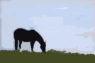
k = 100	k = 10

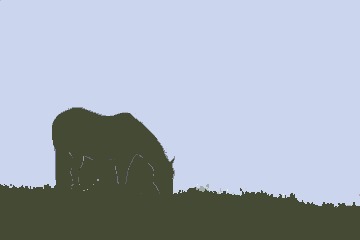We only got two segments with k = 100. Setting k = 10 resulted in smaller but rather noisy segments. felzenzwalb also takes an optional argument min_size - it removes all segments smaller than min_size pixels. (Most methods don’t remove small segments in their core algorithm. We can use the prune_segments method to postprocess the segmentation result and remove small segments.)

segments = felzenszwalb(img, 10, 100)  # removes segments with fewer than 100 pixels
imshow(map(i->segment_means(segments,i), labels_map(segments)))

Acknowledgements

It has been our pleasure to been able to work under the guidance of Tim Holy as part of Google Summer of Code. It has been an incredible learning experience for us. On a number of occasions, whenever we have needed help on issues, the community has been very forthcoming.